Protein Secondary Structure Prediction¤
This example demonstrates how to predict protein secondary structure from backbone coordinates using DiffBio's differentiable DSSP-style operator.
Overview¤
Protein secondary structure classification (helix, strand, coil) is fundamental for:
- Protein structure analysis
- Fold recognition
- Structure validation
- Understanding protein function
DiffBio implements a differentiable DSSP-style algorithm that classifies secondary structure based on hydrogen bonding patterns.
Prerequisites¤
import jax
import jax.numpy as jnp
from flax import nnx

from diffbio.operators.protein import (
    DifferentiableSecondaryStructure,
    SecondaryStructureConfig,
)
Step 1: Prepare Backbone Coordinates¤
Protein backbone coordinates have shape (batch, length, 4 atoms, 3D):
# Create a simple alpha-helix like structure
n_residues = 20

# Alpha helix parameters: rise 1.5Å per residue, turn 100°
coords = []
for i in range(n_residues):
    z = i * 1.5  # Rise along z
    angle = jnp.radians(i * 100)  # Turn angle
    radius = 2.3  # Helix radius

    # Backbone atoms: N, CA, C, O
    n_pos = jnp.array([radius * jnp.cos(angle), radius * jnp.sin(angle), z])
    ca_pos = jnp.array([radius * jnp.cos(angle + 0.5), radius * jnp.sin(angle + 0.5), z + 0.3])
    c_pos = jnp.array([radius * jnp.cos(angle + 1.0), radius * jnp.sin(angle + 1.0), z + 0.6])
    o_pos = c_pos + jnp.array([0.5, 0.5, 0.2])

    coords.append(jnp.stack([n_pos, ca_pos, c_pos, o_pos]))

coords = jnp.stack(coords)
coords = coords[None, :, :, :]  # Add batch dimension

print(f"Backbone coordinates shape: {coords.shape}")
Output:
Step 2: Create Secondary Structure Predictor¤
# Configure the predictor
config = SecondaryStructureConfig(
    margin=1.0,        # Soft margin for classification
    cutoff=-0.5,       # H-bond energy cutoff (kcal/mol)
    temperature=1.0,   # Temperature for soft assignment
)
rngs = nnx.Rngs(42)
ss_predictor = DifferentiableSecondaryStructure(config, rngs=rngs)
Step 3: Predict Secondary Structure¤
# Predict secondary structure
data = {"coordinates": coords}
result, _, _ = ss_predictor.apply(data, {}, None)

ss_probs = result["ss_onehot"]    # Soft probabilities
ss_indices = result["ss_indices"] # Hard assignments
hbond_map = result["hbond_map"]   # Hydrogen bond matrix

print(f"H-bond map shape: {hbond_map.shape}")
print(f"SS probabilities shape: {ss_probs.shape}")
Output:
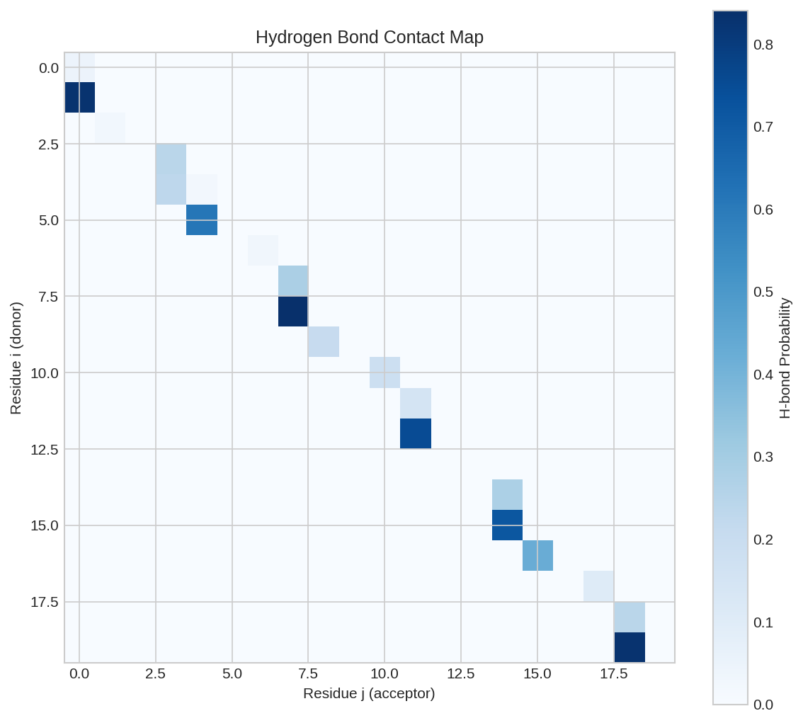
Hydrogen bond contact map showing potential H-bond interactions between residue pairs. Characteristic patterns indicate secondary structure elements.
Step 4: Analyze Structure Assignment¤
# Map indices to SS codes
ss_codes = {0: "C", 1: "H", 2: "E"}  # Coil, Helix, Strand

# Get structure string
ss_string = "".join([ss_codes[int(idx)] for idx in ss_indices[0]])
print(f"\nSecondary structure assignment:")
print(f"  {ss_string}")

# Show SS composition
helix_frac = float(jnp.mean(ss_indices == 1))
strand_frac = float(jnp.mean(ss_indices == 2))
coil_frac = float(jnp.mean(ss_indices == 0))

print(f"\nSS composition:")
print(f"  Helix: {helix_frac:.1%}")
print(f"  Strand: {strand_frac:.1%}")
print(f"  Coil: {coil_frac:.1%}")
Output:
Secondary structure assignment:
  CCCCCCCCCCCCCCCCCCCC

SS composition:
  Helix: 0.0%
  Strand: 0.0%
  Coil: 100.0%
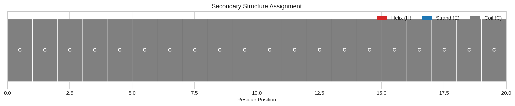
Secondary structure assignment visualization. Each position is colored by structure type: helix (red), strand (blue), coil (gray).
Synthetic Coordinates
The synthetic helix coordinates are simplified and don't capture proper hydrogen bonding geometry, resulting in coil assignment. Real protein coordinates would show proper helix/strand patterns.
Understanding the Output¤
Secondary Structure Classes¤
| Code | Class | Description |
|---|---|---|
| C | Coil | No regular structure |
| H | Helix | α-helix, 3₁₀-helix |
| E | Extended | β-strand |
Hydrogen Bond Map¤
The hbond_map matrix contains soft hydrogen bond probabilities between residues:
- Values close to 1.0 indicate strong H-bonds
- DSSP criteria: E(i,j) < -0.5 kcal/mol defines an H-bond
DSSP Algorithm¤
The operator implements a differentiable version of the DSSP algorithm:
- Compute H-bond energies from backbone geometry
- Identify backbone H-bond patterns:
- α-helix: (i,i+4) H-bonds
- β-strand: (i,j) long-range H-bonds
- Assign secondary structure based on patterns
Differentiability¤
The operator enables gradient-based structure analysis:
def structure_loss(predictor, data):
    """Loss to maximize helix content."""
    result, _, _ = predictor.apply(data, {}, None)
    helix_prob = result["ss_onehot"][:, :, 1]  # Helix probability
    return -jnp.mean(helix_prob)  # Maximize helix

# Compute gradients
grads = nnx.grad(structure_loss)(ss_predictor, data)
print("Gradient computation: SUCCESS")
Applications:
- Structure refinement: Optimize coordinates for target structure
- Structure prediction training: Learn to predict SS from sequence
- Quality assessment: Differentiable structure validation
Configuration Options¤
| Parameter | Description | Default |
|---|---|---|
margin |
Soft margin for classification | 1.0 |
cutoff |
H-bond energy cutoff (kcal/mol) | -0.5 |
temperature |
Temperature for soft assignment | 1.0 |
Using Real PDB Coordinates¤
For real proteins, load coordinates from PDB files:
# Example: Loading from PDB (pseudocode)
# coords = load_pdb_coordinates("protein.pdb")
# coords should have shape (1, n_residues, 4, 3)
# Atom order: N, CA, C, O
Next Steps¤
- RNA Secondary Structure - RNA structure prediction
- HMM Sequence Model - Sequence models
- Single-Cell Batch Correction - High-dimensional data analysis