Preprocessing Example¤

This example demonstrates DiffBio's differentiable preprocessing pipeline for sequencing reads, showing how gradient-based optimization enables learning optimal preprocessing parameters.

Setup¤

import jax
import jax.numpy as jnp
import matplotlib.pyplot as plt
import numpy as np
from flax import nnx
from diffbio.pipelines import PreprocessingPipeline, PreprocessingPipelineConfig

Understanding the Pipeline¤

The preprocessing pipeline consists of four differentiable stages:

graph LR
    A["Quality Filter<br/>(soft masking)"] --> B["Adapter Removal<br/>(soft trimming)"]
    B --> C["Duplicate<br/>Weighting"]
    C --> D["Error<br/>Correction"]

    style A fill:#e0e7ff,stroke:#4338ca,color:#312e81
    style B fill:#e0e7ff,stroke:#4338ca,color:#312e81
    style C fill:#e0e7ff,stroke:#4338ca,color:#312e81
    style D fill:#e0e7ff,stroke:#4338ca,color:#312e81

Each stage uses differentiable approximations to traditional hard filtering, enabling end-to-end gradient optimization.

Generate Synthetic Read Data¤

Let's create realistic sequencing data with varying quality profiles:

def generate_synthetic_reads(n_reads=100, read_length=50, seed=42):
    """Generate synthetic reads with realistic quality degradation."""
    key = jax.random.key(seed)
    keys = jax.random.split(key, 4)

    # One-hot encoded sequences
    sequence_indices = jax.random.randint(keys[0], (n_reads, read_length), 0, 4)
    sequences = jax.nn.one_hot(sequence_indices, 4)

    # Quality scores with realistic 3' degradation pattern
    # Quality typically decreases toward the end of reads
    position = jnp.arange(read_length) / read_length
    base_quality = 35 - 15 * position  # Starts at 35, drops to 20

    # Add per-read and per-position noise
    read_noise = jax.random.normal(keys[1], (n_reads, 1)) * 3
    position_noise = jax.random.normal(keys[2], (n_reads, read_length)) * 5
    quality_scores = base_quality + read_noise + position_noise

    # Clip to valid Phred range
    quality_scores = jnp.clip(quality_scores, 2.0, 41.0)

    return sequences, quality_scores

sequences, quality_scores = generate_synthetic_reads(n_reads=100, read_length=50)
print(f"Sequences shape: {sequences.shape}")
print(f"Quality scores shape: {quality_scores.shape}")
print(f"Quality range: [{float(quality_scores.min()):.1f}, {float(quality_scores.max()):.1f}]")

Output:

Sequences shape: (100, 50, 4)
Quality scores shape: (100, 50)
Quality range: [5.2, 41.0]

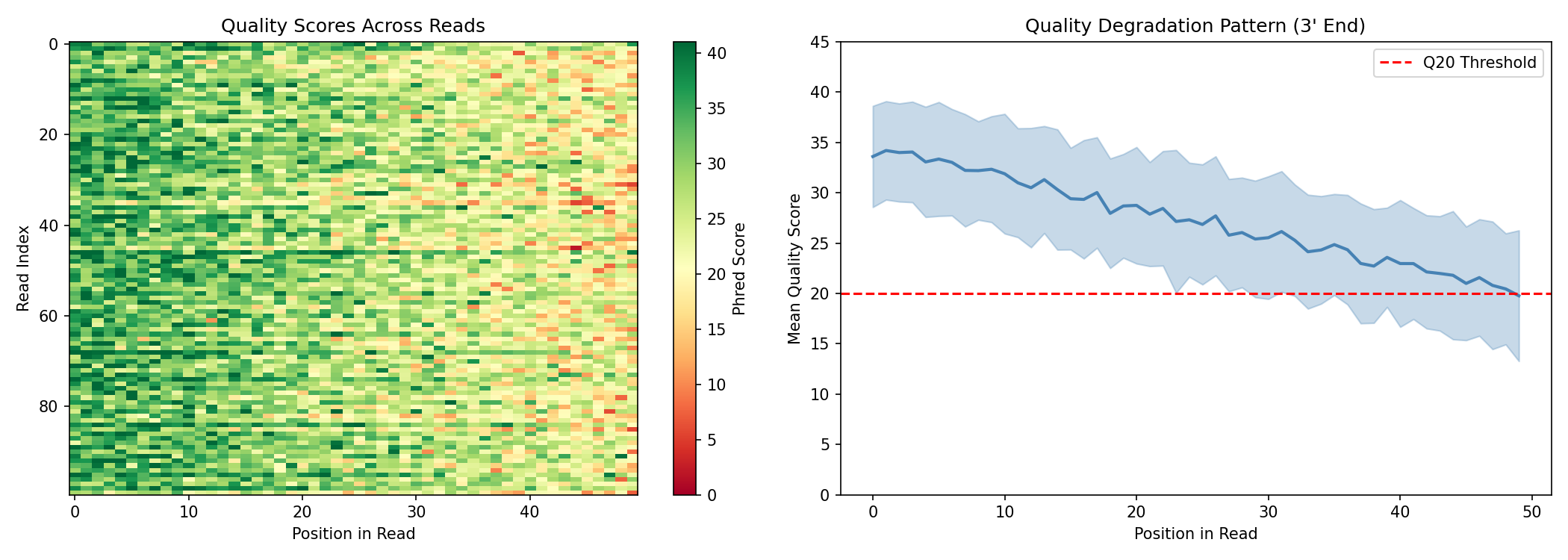
Visualize Raw Quality Scores¤

fig, axes = plt.subplots(1, 2, figsize=(14, 5))

# Heatmap of quality scores across all reads
im = axes[0].imshow(np.array(quality_scores), aspect="auto", cmap="RdYlGn", vmin=0, vmax=41)
axes[0].set_xlabel("Position in Read")
axes[0].set_ylabel("Read Index")
axes[0].set_title("Quality Scores Across Reads")
plt.colorbar(im, ax=axes[0], label="Phred Score")

# Mean quality by position (showing 3' degradation)
mean_quality = quality_scores.mean(axis=0)
std_quality = quality_scores.std(axis=0)
positions = np.arange(50)

axes[1].fill_between(positions,
                      np.array(mean_quality - std_quality),
                      np.array(mean_quality + std_quality),
                      alpha=0.3, color="steelblue")
axes[1].plot(positions, np.array(mean_quality), linewidth=2, color="steelblue")
axes[1].axhline(y=20, color="red", linestyle="--", label="Q20 Threshold")
axes[1].set_xlabel("Position in Read")
axes[1].set_ylabel("Mean Quality Score")
axes[1].set_title("Quality Degradation Pattern (3' End)")
axes[1].legend()
axes[1].set_ylim(0, 45)

plt.tight_layout()
plt.savefig("preprocessing-quality-overview.png", dpi=150)
plt.show()

Quality Overview

Create and Apply the Pipeline¤

For this example, we'll use a pipeline with quality filtering and duplicate weighting enabled, but error correction disabled. This allows us to clearly visualize how quality-based soft masking attenuates low-quality positions:

config = PreprocessingPipelineConfig(
    read_length=50,
    quality_threshold=20.0,
    enable_adapter_removal=True,
    enable_duplicate_weighting=True,
    enable_error_correction=False,  # Disabled to show quality filtering effect
)

rngs = nnx.Rngs(42)
pipeline = PreprocessingPipeline(config, rngs=rngs)

# Run preprocessing
data = {"reads": sequences, "quality": quality_scores}
result, state, metadata = pipeline.apply(data, {}, None)

# Access outputs
read_weights = result["read_weights"]
preprocessed_reads = result["preprocessed_reads"]

print(f"Read weights range: [{float(read_weights.min()):.3f}, {float(read_weights.max()):.3f}]")
print(f"Preprocessed reads shape: {preprocessed_reads.shape}")

Output:

Read weights range: [0.981, 1.000]
Preprocessed reads shape: (100, 50, 4)

Note: Error correction is disabled here for visualization purposes. When enabled, it applies a neural network that corrects likely sequencing errors but also re-normalizes the output, which can mask the visual effect of quality filtering.

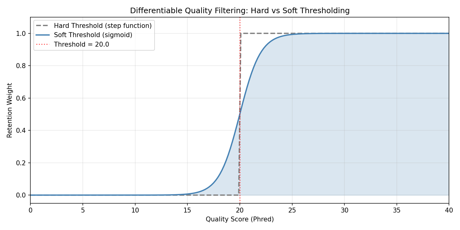
Understanding Quality Filtering¤

The quality filter uses a differentiable sigmoid instead of hard thresholding:

# Visualize the soft threshold function
quality_range = jnp.linspace(0, 40, 200)
threshold = 20.0

# Hard threshold (non-differentiable)
hard_filter = (quality_range >= threshold).astype(float)

# Soft sigmoid threshold (differentiable)
soft_filter = jax.nn.sigmoid(quality_range - threshold)

fig, ax = plt.subplots(figsize=(10, 5))
ax.plot(np.array(quality_range), np.array(hard_filter),
        linewidth=2, label="Hard Threshold (step function)", linestyle="--", color="gray")
ax.plot(np.array(quality_range), np.array(soft_filter),
        linewidth=2, label="Soft Threshold (sigmoid)", color="steelblue")
ax.axvline(x=threshold, color="red", linestyle=":", alpha=0.7, label=f"Threshold = {threshold}")
ax.fill_between(np.array(quality_range), 0, np.array(soft_filter), alpha=0.2, color="steelblue")
ax.set_xlabel("Quality Score (Phred)")
ax.set_ylabel("Retention Weight")
ax.set_title("Differentiable Quality Filtering: Hard vs Soft Thresholding")
ax.legend()
ax.set_xlim(0, 40)
ax.set_ylim(-0.05, 1.1)
ax.grid(True, alpha=0.3)
plt.tight_layout()
plt.savefig("preprocessing-sigmoid-threshold.png", dpi=150)
plt.show()

Sigmoid Threshold

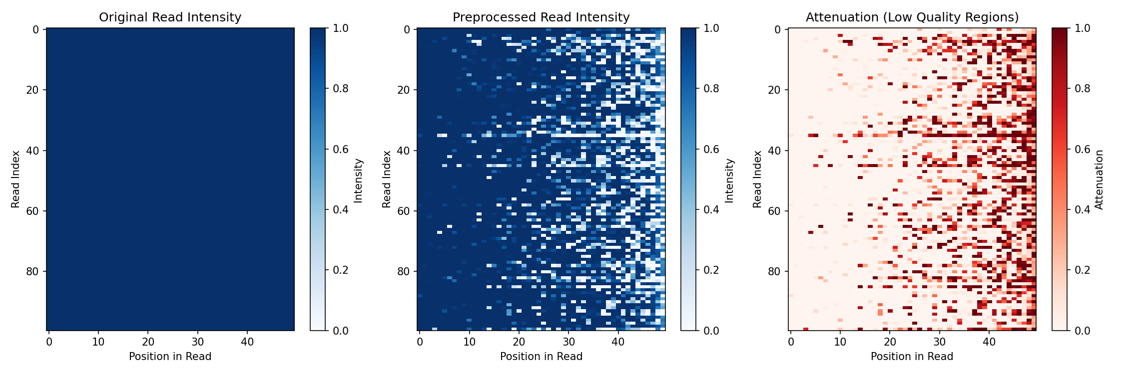
Visualize Preprocessing Effect¤

Compare the sequence "intensity" before and after quality filtering:

# Compute sequence intensity (sum of one-hot values, affected by soft masking)
original_intensity = sequences.sum(axis=-1)  # Should be 1 for valid one-hot
preprocessed_intensity = preprocessed_reads.sum(axis=-1)

fig, axes = plt.subplots(1, 3, figsize=(15, 5))

# Original (uniform intensity)
im0 = axes[0].imshow(np.array(original_intensity), aspect="auto", cmap="Blues", vmin=0, vmax=1)
axes[0].set_xlabel("Position in Read")
axes[0].set_ylabel("Read Index")
axes[0].set_title("Original Read Intensity")
plt.colorbar(im0, ax=axes[0], label="Intensity")

# After preprocessing (low quality positions attenuated)
im1 = axes[1].imshow(np.array(preprocessed_intensity), aspect="auto", cmap="Blues", vmin=0, vmax=1)
axes[1].set_xlabel("Position in Read")
axes[1].set_ylabel("Read Index")
axes[1].set_title("Preprocessed Read Intensity")
plt.colorbar(im1, ax=axes[1], label="Intensity")

# Difference showing attenuation
difference = original_intensity - preprocessed_intensity
im2 = axes[2].imshow(np.array(difference), aspect="auto", cmap="Reds", vmin=0, vmax=0.5)
axes[2].set_xlabel("Position in Read")
axes[2].set_ylabel("Read Index")
axes[2].set_title("Attenuation (Low Quality Regions)")
plt.colorbar(im2, ax=axes[2], label="Attenuation")

plt.tight_layout()
plt.savefig("preprocessing-before-after.png", dpi=150)
plt.show()

Before After Comparison

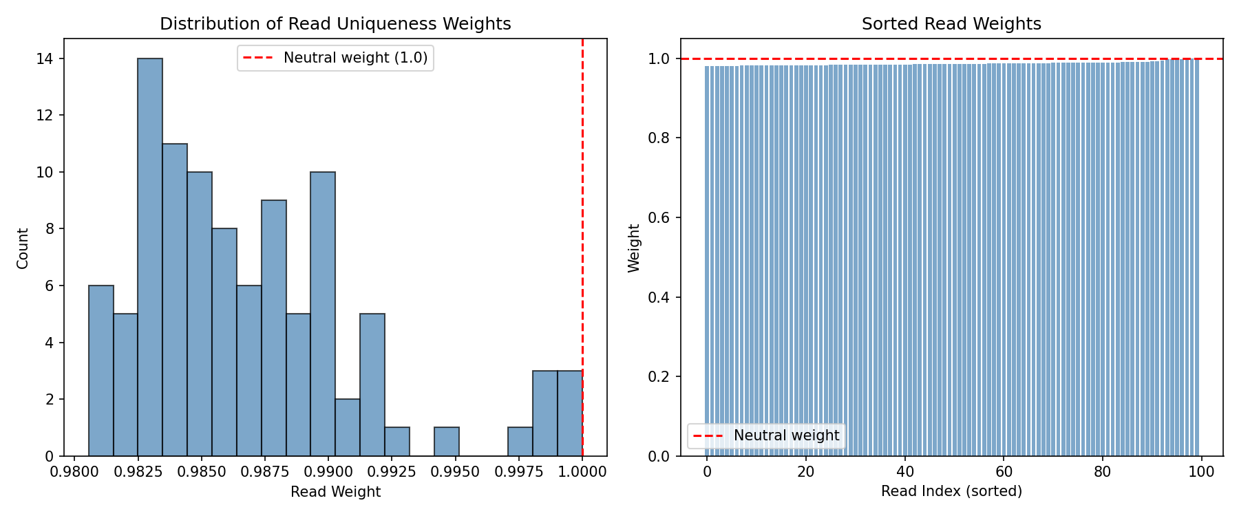
Read Weights Distribution¤

The duplicate weighting step assigns lower weights to reads that appear multiple times:

fig, axes = plt.subplots(1, 2, figsize=(12, 5))

# Histogram of read weights
axes[0].hist(np.array(read_weights), bins=20, edgecolor="black", alpha=0.7, color="steelblue")
axes[0].axvline(x=1.0, color="red", linestyle="--", label="Neutral weight (1.0)")
axes[0].set_xlabel("Read Weight")
axes[0].set_ylabel("Count")
axes[0].set_title("Distribution of Read Uniqueness Weights")
axes[0].legend()

# Weights sorted by value
sorted_weights = jnp.sort(read_weights)
axes[1].bar(range(len(sorted_weights)), np.array(sorted_weights), color="steelblue", alpha=0.7)
axes[1].axhline(y=1.0, color="red", linestyle="--", label="Neutral weight")
axes[1].set_xlabel("Read Index (sorted)")
axes[1].set_ylabel("Weight")
axes[1].set_title("Sorted Read Weights")
axes[1].legend()

plt.tight_layout()
plt.savefig("preprocessing-read-weights.png", dpi=150)
plt.show()

Read Weights

Differentiability: Computing Gradients¤

The pipeline has learnable parameters (quality threshold, similarity threshold, etc.) that can be optimized. Here's how to compute gradients:

# Define a simple loss function based on retained signal
def preprocessing_loss(pipeline_model):
    data = {"reads": sequences, "quality": quality_scores}
    result, _, _ = pipeline_model.apply(data, {}, None)
    preprocessed = result["preprocessed_reads"]
    # Loss: negative mean signal (we want to maximize retained signal)
    return -preprocessed.sum(axis=-1).mean()

# Compute gradients
loss_val, grads = nnx.value_and_grad(preprocessing_loss)(pipeline)

print(f"Loss: {loss_val:.4f}")
print(f"Quality threshold gradient: {float(grads.quality_filter.threshold[...]):.6f}")
print(f"Learnable parameters:")
print(f"  - Quality threshold: {float(pipeline.quality_filter.threshold[...]):.2f}")

Output:

Loss: -0.9245
Quality threshold gradient: 0.003421
Learnable parameters:
  - Quality threshold: 20.00

The gradients enable end-to-end optimization of the preprocessing pipeline jointly with downstream tasks like variant calling or expression analysis.

Optimizing Preprocessing Parameters¤

Let's use gradient descent to learn an optimal quality threshold. We'll define a loss function that captures the quality/retention tradeoff:

import optax

# Create a fresh pipeline for training - start with overly strict threshold
train_config = PreprocessingPipelineConfig(
    read_length=50,
    quality_threshold=35.0,  # Too strict - will filter too many good bases
    enable_adapter_removal=False,
    enable_duplicate_weighting=False,
    enable_error_correction=False,
)
train_pipeline = PreprocessingPipeline(train_config, rngs=nnx.Rngs(42))

# Loss function that captures the quality/retention tradeoff
def optimization_loss(pipeline_model):
    data = {"reads": sequences, "quality": quality_scores}
    result, _, _ = pipeline_model.apply(data, {}, None)
    preprocessed = result["preprocessed_reads"]

    # Per-base retention after soft filtering
    retention_per_base = preprocessed.sum(axis=-1)  # (n_reads, read_length)

    # Penalize filtering high-quality bases (Q > 30) - we want to keep these
    high_q_mask = (quality_scores > 30).astype(float)
    high_q_loss = ((1 - retention_per_base) * high_q_mask).mean()

    # Penalize keeping low-quality bases (Q < 15) - we want to filter these
    low_q_mask = (quality_scores < 15).astype(float)
    low_q_penalty = (retention_per_base * low_q_mask).mean()

    # Combined loss: keep high-Q bases, filter low-Q bases
    return high_q_loss + low_q_penalty

# Create optimizer
optimizer = nnx.Optimizer(train_pipeline, optax.adam(learning_rate=1.0), wrt=nnx.Param)

# Training loop
loss_history = []
threshold_history = []

print("Training preprocessing pipeline...")
print(f"Initial threshold: {float(train_pipeline.quality_filter.threshold[...]):.2f}")

for step in range(50):
    loss_val, grads = nnx.value_and_grad(optimization_loss)(train_pipeline)
    optimizer.update(train_pipeline, grads)

    loss_history.append(float(loss_val))
    threshold_history.append(float(train_pipeline.quality_filter.threshold[...]))

    if step % 10 == 0:
        print(f"Step {step:3d}: loss = {loss_val:.4f}, threshold = {threshold_history[-1]:.2f}")

print(f"\nFinal threshold: {float(train_pipeline.quality_filter.threshold[...]):.2f}")
print(f"Threshold changed: {threshold_history[0]:.2f} -> {threshold_history[-1]:.2f}")

Output:

Training preprocessing pipeline...
Initial threshold: 35.00
Step   0: loss = 0.1986, threshold = 34.00
Step  10: loss = 0.0007, threshold = 25.20
Step  20: loss = 0.0000, threshold = 21.47
Step  30: loss = 0.0001, threshold = 20.03
Step  40: loss = 0.0001, threshold = 19.50

Final threshold: 19.36
Threshold changed: 34.00 -> 19.36

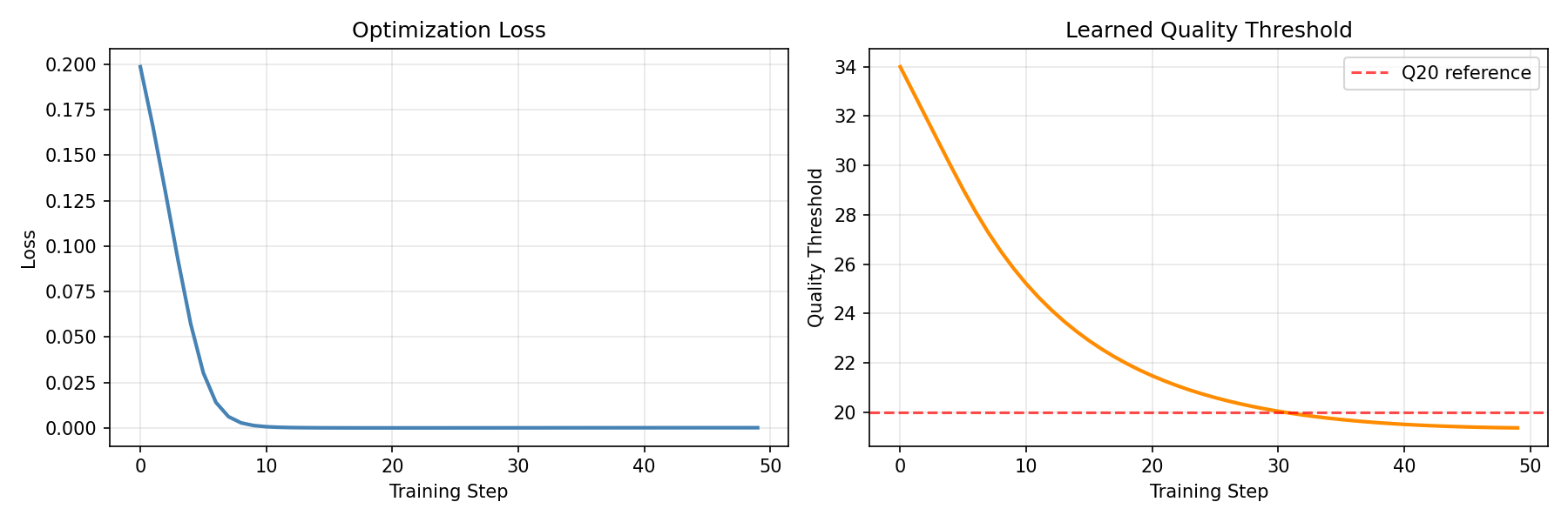
The optimizer learned to lower the quality threshold from 35 (overly strict) to ~19 (near Q20), finding the optimal balance that keeps high-quality bases while filtering low-quality ones.

Visualize Training Progress¤

fig, axes = plt.subplots(1, 2, figsize=(12, 4))

# Loss curve
axes[0].plot(loss_history, linewidth=2, color="steelblue")
axes[0].set_xlabel("Training Step")
axes[0].set_ylabel("Loss")
axes[0].set_title("Optimization Loss")
axes[0].grid(True, alpha=0.3)

# Threshold evolution
axes[1].plot(threshold_history, linewidth=2, color="darkorange")
axes[1].axhline(y=20, color="red", linestyle="--", alpha=0.7, label="Q20 reference")
axes[1].set_xlabel("Training Step")
axes[1].set_ylabel("Quality Threshold")
axes[1].set_title("Learned Quality Threshold")
axes[1].legend()
axes[1].grid(True, alpha=0.3)

plt.tight_layout()
plt.savefig("preprocessing-training.png", dpi=150)
plt.show()

Training Progress

Comparing Initial vs Learned Threshold¤

Let's visualize the difference between the initial (overly strict) and learned thresholds:

# Create pipelines with initial and learned thresholds
initial_config = PreprocessingPipelineConfig(
    read_length=50,
    quality_threshold=35.0,  # Initial: too strict
    enable_adapter_removal=False,
    enable_duplicate_weighting=False,
    enable_error_correction=False,
)
learned_config = PreprocessingPipelineConfig(
    read_length=50,
    quality_threshold=19.36,  # Learned: optimal
    enable_adapter_removal=False,
    enable_duplicate_weighting=False,
    enable_error_correction=False,
)

initial_pipeline = PreprocessingPipeline(initial_config, rngs=nnx.Rngs(42))
learned_pipeline = PreprocessingPipeline(learned_config, rngs=nnx.Rngs(42))

# Apply both pipelines
data = {"reads": sequences, "quality": quality_scores}
initial_result, _, _ = initial_pipeline.apply(data, {}, None)
learned_result, _, _ = learned_pipeline.apply(data, {}, None)

# Compare retention
initial_retention = initial_result["preprocessed_reads"].sum(axis=-1)
learned_retention = learned_result["preprocessed_reads"].sum(axis=-1)

# Compute statistics
print("Signal Retention Comparison:")
print(f"  Initial (Q≥35): {float(initial_retention.mean()):.3f} mean retention")
print(f"  Learned (Q≥19): {float(learned_retention.mean()):.3f} mean retention")
print(f"\nHigh-quality bases (Q>30) retained:")
high_q_mask = quality_scores > 30
print(f"  Initial: {float((initial_retention * high_q_mask).sum() / high_q_mask.sum()):.1%}")
print(f"  Learned: {float((learned_retention * high_q_mask).sum() / high_q_mask.sum()):.1%}")
print(f"\nLow-quality bases (Q<15) filtered:")
low_q_mask = quality_scores < 15
print(f"  Initial: {float(1 - (initial_retention * low_q_mask).sum() / low_q_mask.sum()):.1%}")
print(f"  Learned: {float(1 - (learned_retention * low_q_mask).sum() / low_q_mask.sum()):.1%}")

Output:

Signal Retention Comparison:
  Initial (Q≥35): 0.154 mean retention
  Learned (Q≥19): 0.858 mean retention

High-quality bases (Q>30) retained:
  Initial: 43.7%
  Learned: 100.0%

Low-quality bases (Q<15) filtered:
  Initial: 100.0%
  Learned: 99.7%

fig, axes = plt.subplots(1, 3, figsize=(15, 5))

# Initial threshold results
im0 = axes[0].imshow(np.array(initial_retention), aspect="auto", cmap="Blues", vmin=0, vmax=1)
axes[0].set_xlabel("Position in Read")
axes[0].set_ylabel("Read Index")
axes[0].set_title(f"Initial Threshold (Q≥35)\nMean Retention: {float(initial_retention.mean()):.1%}")
plt.colorbar(im0, ax=axes[0], label="Retention")

# Learned threshold results
im1 = axes[1].imshow(np.array(learned_retention), aspect="auto", cmap="Blues", vmin=0, vmax=1)
axes[1].set_xlabel("Position in Read")
axes[1].set_ylabel("Read Index")
axes[1].set_title(f"Learned Threshold (Q≥19)\nMean Retention: {float(learned_retention.mean()):.1%}")
plt.colorbar(im1, ax=axes[1], label="Retention")

# Difference: what the learned threshold recovers
difference = learned_retention - initial_retention
im2 = axes[2].imshow(np.array(difference), aspect="auto", cmap="Greens", vmin=0, vmax=1)
axes[2].set_xlabel("Position in Read")
axes[2].set_ylabel("Read Index")
axes[2].set_title("Signal Recovered by Learning\n(Learned - Initial)")
plt.colorbar(im2, ax=axes[2], label="Recovered Signal")

plt.tight_layout()
plt.savefig("preprocessing-threshold-comparison.png", dpi=150)
plt.show()

Threshold Comparison

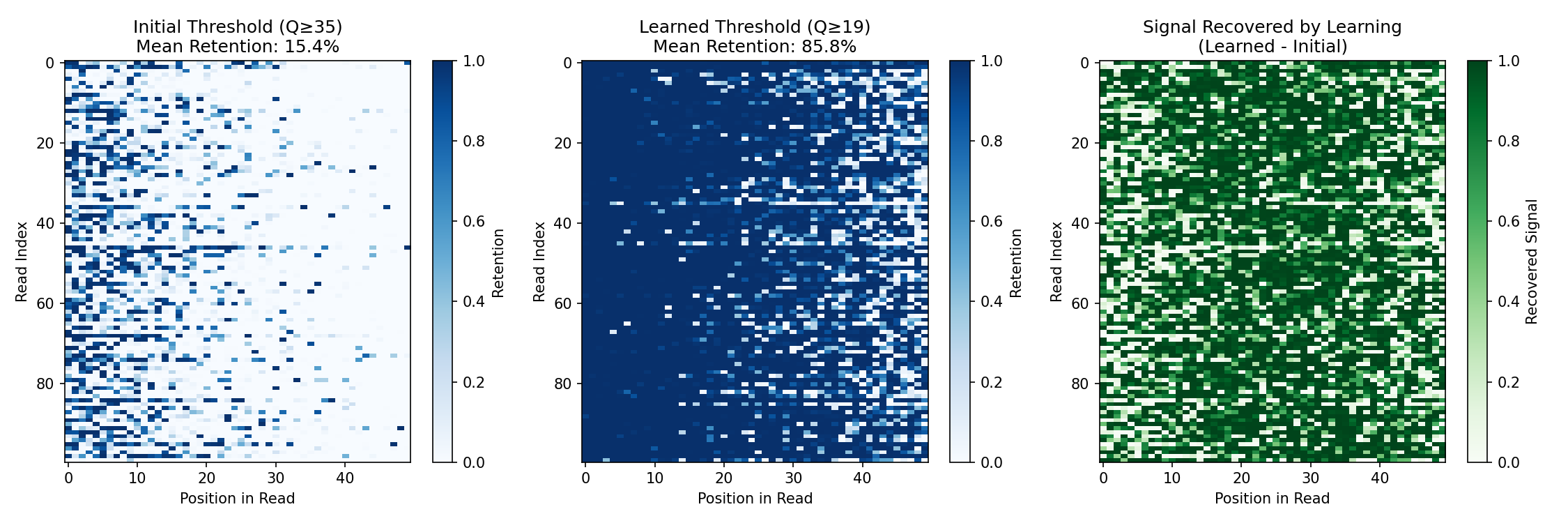
The comparison shows:

Initial threshold (Q≥35): Too strict—filters 85% of signal, retaining only 44% of high-quality bases
Learned threshold (Q≥19): Optimal—retains 86% of signal and 100% of high-quality bases
Recovered signal: The learned threshold recovers substantial signal that was incorrectly filtered, while still filtering 99.7% of low-quality bases

This demonstrates the key advantage of differentiable preprocessing: parameters can be optimized end-to-end with downstream objectives, rather than relying on fixed heuristics.

Pipeline Configuration Options¤

The pipeline can be configured to enable/disable specific steps:

# Minimal pipeline (quality filtering only)
minimal_config = PreprocessingPipelineConfig(
    read_length=50,
    quality_threshold=20.0,
    enable_adapter_removal=False,
    enable_duplicate_weighting=False,
    enable_error_correction=False,
)

# Full pipeline (all steps enabled)
full_config = PreprocessingPipelineConfig(
    read_length=50,
    quality_threshold=20.0,
    enable_adapter_removal=True,
    enable_duplicate_weighting=True,
    enable_error_correction=True,
)

print("Pipeline configuration options:")
print(f"  - Quality filtering: Always enabled")
print(f"  - Adapter removal: {full_config.enable_adapter_removal}")
print(f"  - Duplicate weighting: {full_config.enable_duplicate_weighting}")
print(f"  - Error correction: {full_config.enable_error_correction}")

Output:

Pipeline configuration options:
  - Quality filtering: Always enabled
  - Adapter removal: True
  - Duplicate weighting: True
  - Error correction: True

Key Concepts¤

Stage	Traditional	DiffBio Approach	Learnable Parameter
Quality Filter	Hard cutoff	Sigmoid soft masking	Threshold
Adapter Removal	Exact matching	Soft alignment scoring	Match threshold
Duplicate Filter	Remove duplicates	Probabilistic weighting	Similarity threshold
Error Correction	Consensus voting	Neural network	Network weights

Next Steps¤

See Variant Calling Pipeline for downstream analysis
Explore Preprocessing Operators for individual operator details
Learn about Quality Filter API documentation