DiffBio Example Documentation Design Guide¤
This guide defines how to design, write, maintain, and review DiffBio examples. It is specific to DiffBio's current runtime and contributor contract:
- reader-facing tutorial examples are dual-format
.pyand.ipynbpairs - verification and maintenance utilities under
examples/may remain.pyonly - repository workflows use
uv - examples target JAX and Flax NNX on the datarax pipeline framework
- operators follow the
OperatorModule.apply()contract from datarax - backend behavior follows JAX defaults instead of custom CUDA forcing
- contributor-facing example docs live under
docs/examples/
Purpose¤
DiffBio examples must do three jobs at once:
- Teach a concrete bioinformatics concept through differentiable computation.
- Demonstrate the current supported DiffBio API and ecosystem integration.
- Run successfully as real code, not documentation theater.
An example is successful only when all three are true.
Scope¤
This guide applies to:
- runnable example sources under
examples/ - paired example notebooks under
examples/ - example documentation pages under
docs/examples/ - example templates under
docs/examples/templates/
It also informs contributor-facing documentation in:
CONTRIBUTING.mddocs/development/contributing.mdexamples/README.md
Design Principles¤
Teach Through Real Execution¤
Examples should run end to end with the commands shown in the docs. Prefer small working pipelines over aspirational pseudo-workflows. Every code block should be copy-pasteable and produce the shown output.
However, readers should not need to run the code to learn from the example. The docs page must embed all visual outputs (figures, plots) and key textual results directly. A reader browsing the documentation should see exactly what the example produces — training curves, scatter plots, metric tables — without touching a terminal.
Prefer Present-Tense API Guidance¤
Document the current supported DiffBio surface. Avoid transitional language and avoid teaching historical implementation details.
Progressive Disclosure¤
Each example should start with the smallest useful path, then add complexity in clear stages:
- environment and prerequisites
- imports and configuration
- data creation or loading (synthetic or via
AnnDataSource) - operator construction and
apply() - inspection of outputs (shapes and key scalar values)
- visualization of results (at least one matplotlib figure, saved to
docs/assets/examples/) - gradient flow verification (differentiability is DiffBio's value proposition)
- JIT compilation verification
- experiments with parameter sweeps (each sweep produces a figure)
Differentiability First¤
Every operator example must include a gradient flow demonstration. This is DiffBio's core value proposition — showing that bioinformatics pipelines are end-to-end differentiable. At minimum, show:
# Verify gradient flow
def loss_fn(data):
    result, _, _ = operator.apply(data, {}, None, None)
    return result["output_key"].sum()

grad = jax.grad(loss_fn)(data)
print(f"Gradient shape: {grad['counts'].shape}")
print(f"Gradient is non-zero: {jnp.any(grad['counts'] != 0)}")
JIT Compilation Demo¤
Every operator example should show JIT compilation works:
# JIT-compiled forward pass
@jax.jit
def jit_apply(data):
    result, _, _ = operator.apply(data, {}, None, None)
    return result

result = jit_apply(data)
CPU-Safe by Default¤
Examples should run on CPU unless the example is inherently GPU-bound. GPU use is an optimization path, not an excuse for unclear setup.
GPU Requirements Must Be Explicit¤
If an example requires GPU, say so at the top and provide a direct verification step with:
If GPU is optional, say that clearly and avoid device forcing logic inside the example.
Source of Truth Lives in the Example Pair¤
For dual-format tutorial examples, the runnable .py and .ipynb pair is the
technical source of truth. The corresponding docs/examples/... page explains
the example, but should not drift from the actual source files.
Documentation Architecture¤
Every substantial reader-facing tutorial example should have three aligned artifacts:
examples/.../example_name.pyThe runnable Jupytext-backed Python source.examples/.../example_name.ipynbThe paired notebook generated from the Python source.docs/examples/.../example-name.mdThe reader-facing documentation page.
Use this split intentionally:
.pyis the easiest source to review and refactor..ipynbsupports notebook-first exploration..mdexplains context, expected outcomes, and navigation.
Utility scripts under examples/ are different. If the file exists to verify,
benchmark, or maintain the example surface rather than teach a workflow, it can
stay as a Python-only script with no paired notebook.
Location Strategy¤
Put examples where users will expect them, organized by DiffBio's domain structure:
examples/basics/for foundational patterns (configs, operators, data flow)examples/singlecell/for single-cell analysis workflowsexamples/alignment/for sequence alignment examplesexamples/variant/for variant calling examplesexamples/drug_discovery/for molecular property predictionexamples/multiomics/for multi-omics integrationexamples/epigenomics/for chromatin and peak analysisexamples/pipelines/for end-to-end pipeline compositionexamples/ecosystem/for datarax/artifex/calibrax/opifex integration demos
Put documentation under the corresponding docs/examples/ section so the docs
match the runnable source domain.
Dual-Format Workflow¤
Reader-facing tutorial examples should be maintained as Jupytext pairs. Use the repo tool, not ad hoc manual notebook edits.
Create a New Example¤
Start from:
docs/examples/templates/example_template.py
The paired .ipynb is generated from the .py via scripts/jupytext_converter.py (see Sync the Pair below).
Sync the Pair¤
Use the project's jupytext converter script:
Validate the Pair¤
Use:
source ./activate.sh
uv run python scripts/jupytext_converter.py validate examples/path/to/
uv run python examples/path/to/example.py
The Python file should remain the main review surface. The notebook should be regenerated from it rather than hand-edited independently.
Do not create notebook pairs for verification or maintenance scripts such as
examples/verify_examples.py.
Runtime and Backend Contract¤
Activation¤
Always show:
Keep the repository-relative ./ prefix when documenting activation.
Execution¤
Run examples through uv:
Do not document direct python ... commands as the primary path.
Backend Selection¤
Let JAX select the best available backend by default. Do not teach or embed:
- hard-coded multi-platform fallback lists
- system CUDA toolkit paths
- custom CUDA library path management
Device Statements¤
At the top of each example page, state one of:
CPU-compatibleGPU-optionalGPU-required
If GPU-required, include the activation command. If CPU-compatible, say so explicitly.
Code Standards for Examples¤
Use the Supported Runtime Surface¤
Examples should prefer public imports:
# Operators
from diffbio.operators.singlecell.trajectory import (
    DifferentiablePseudotime,
    PseudotimeConfig,
)

# Losses
from diffbio.losses.singlecell_losses import ShannonDiversityLoss

# Core utilities
from diffbio.core.graph_utils import compute_pairwise_distances

# Ecosystem
from calibrax.metrics.functional.clustering import silhouette_score
from artifex.generative_models.core.losses.divergence import gaussian_kl_divergence
Avoid reaching through private or transitional paths when a supported top-level surface exists.
Use Flax NNX¤
DiffBio examples should use Flax NNX patterns consistently:
nnx.Modulennx.Rngs- explicit RNG flow
nnx.Paramfor learnable parametersnnx.relu,nnx.gelufor activations (notjax.nn.*)
Use Typed Configs¤
Prefer the frozen dataclass configuration model from datarax:
config = PseudotimeConfig(
    n_neighbors=15,
    n_diffusion_components=10,
    root_cell_index=0,
)
operator = DifferentiablePseudotime(config, rngs=nnx.Rngs(42))
Follow the apply() Contract¤
All operator examples must use the standard apply() signature:
Where:
- data is a dict of JAX arrays
- state is an empty dict {} for stateless operators
- metadata is None for simple cases
- The result is {**input_data, "new_keys": new_values}
Synthetic Data Over Real Data¤
Examples should generate synthetic data rather than requiring external downloads. This keeps examples self-contained and fast. Use JAX random for data generation:
For more realistic synthetic data, use DifferentiableSimulator:
Keep Side Effects Explicit¤
Examples may print or log progress because they are educational artifacts, but they should not mutate global backend state, modify tracked repo files, or depend on hidden shell state.
Avoid Fake Code¤
Do not include placeholder commands, nonexistent files, or invented outputs. If a section is conceptual, label it as conceptual. If code is runnable, make it actually runnable.
DiffBio-Specific Example Patterns¤
The Standard Operator Example¤
Every operator example follows this skeleton. Note the required visualization
cell after the operator run, and the plt.savefig() call that writes the
figure to the docs assets directory.
# %% [markdown]
# # Operator Name
# Brief description of what this operator does.

# %% [markdown]
# ## Setup

# %%
import jax
import jax.numpy as jnp
import matplotlib.pyplot as plt
from flax import nnx

from diffbio.operators.domain.module import OperatorClass, OperatorConfig

# %% [markdown]
# ## Configuration

# %%
config = OperatorConfig(
    param1=value1,
    param2=value2,
)
operator = OperatorClass(config, rngs=nnx.Rngs(42))

# %% [markdown]
# ## Create Synthetic Data

# %%
key = jax.random.key(0)
data = {"counts": jax.random.poisson(key, jnp.ones((50, 100)) * 3.0)}
print(f"Input shape: {data['counts'].shape}")

# %% [markdown]
# ## Run the Operator

# %%
result, state, metadata = operator.apply(data, {}, None, None)
for key_name, value in result.items():
    if hasattr(value, 'shape'):
        print(f"  {key_name}: {value.shape}")

# %%
# Visualize the output
fig, ax = plt.subplots(figsize=(7, 4))
ax.imshow(result["output_key"][:20, :], aspect="auto", cmap="viridis")
ax.set_xlabel("Feature")
ax.set_ylabel("Sample")
ax.set_title("Operator Output")
plt.colorbar(ax.images[0], ax=ax, label="Value")
plt.tight_layout()
plt.savefig(
    "docs/assets/examples/domain/operator_name_output.png",
    dpi=150, bbox_inches="tight",
)
plt.show()

# %% [markdown]
# ## Verify Differentiability

# %%
def loss_fn(input_data):
    result, _, _ = operator.apply(input_data, {}, None, None)
    return result["output_key"].sum()

grad = jax.grad(loss_fn)(data)
print(f"Gradient shape: {grad['counts'].shape}")
print(f"Gradient is non-zero: {bool(jnp.any(grad['counts'] != 0))}")
print(f"Gradient is finite: {bool(jnp.all(jnp.isfinite(grad['counts'])))}")

# %% [markdown]
# ## JIT Compilation

# %%
jit_apply = jax.jit(lambda d: operator.apply(d, {}, None, None))
result_jit, _, _ = jit_apply(data)
print(f"JIT output matches: {bool(jnp.allclose(result['output_key'], result_jit['output_key']))}")

# %% [markdown]
# ## Experiments

# %%
# Sweep a key parameter and visualize the effect
param_values = [0.1, 0.5, 1.0, 5.0]
metric_values = []
for val in param_values:
    cfg = OperatorConfig(param1=val)
    op = OperatorClass(cfg, rngs=nnx.Rngs(42))
    res, _, _ = op.apply(data, {}, None, None)
    metric_values.append(float(res["output_key"].mean()))

fig, ax = plt.subplots(figsize=(6, 4))
ax.plot(param_values, metric_values, "o-", linewidth=2, markersize=7)
ax.set_xlabel("param1")
ax.set_ylabel("Mean Output")
ax.set_title("Effect of param1 on Output")
plt.tight_layout()
plt.savefig(
    "docs/assets/examples/domain/operator_name_sweep.png",
    dpi=150, bbox_inches="tight",
)
plt.show()
The Pipeline Composition Example¤
Shows how multiple operators chain:
# Step 1: Normalize
norm_result, _, _ = normalizer.apply(data, {}, None, None)

# Step 2: Impute (uses normalized output)
impute_data = {"counts": norm_result["normalized"]}
impute_result, _, _ = imputer.apply(impute_data, {}, None, None)

# Step 3: Trajectory (uses imputed output)
traj_data = {"embeddings": impute_result["imputed_counts"]}
traj_result, _, _ = pseudotime.apply(traj_data, {}, None, None)
The Ecosystem Integration Example¤
Shows how DiffBio connects to datarax/artifex/calibrax/opifex:
# calibrax metrics for evaluation
from calibrax.metrics.functional.clustering import silhouette_score
score = silhouette_score(latent, labels)

# artifex losses for training
from artifex.generative_models.core.losses.divergence import gaussian_kl_divergence
kl = gaussian_kl_divergence(mean, logvar, reduction="sum")

# opifex for multi-task balancing
from opifex.core.physics.gradnorm import GradNormBalancer
Writing the Companion Docs Page¤
The docs page exists so readers can understand an example without running the code. A reader browsing the documentation should see the key figures, expected outputs, and explanations directly on the page. This means:
- every figure produced by the example must be embedded in the docs page
- every key textual output must appear in a fenced output block
- code excerpts show the essential 5-10 lines, not the entire file
Every docs/examples/... page should include:
- what the example demonstrates
- runtime estimate
- device requirements
- prerequisites (which DiffBio modules are needed)
- exact execution command
- a short map of the major sections
- a few key code excerpts with commentary
- embedded figures from
docs/assets/examples/...with alt text - expected textual output in fenced code blocks
- related examples
Good top-of-page structure:
# Example Title
**Duration:** 10 min | **Level:** Intermediate | **Device:** CPU-compatible
## Overview
[1-3 sentences: what this example does and why it matters.]
## Quick Start
source ./activate.sh
uv run python examples/singlecell/clustering.py
## Key Code
[5-10 line excerpt of the apply() call with a sentence of context.]
## Results
[Embedded figure + interpretation sentence + textual output block.]
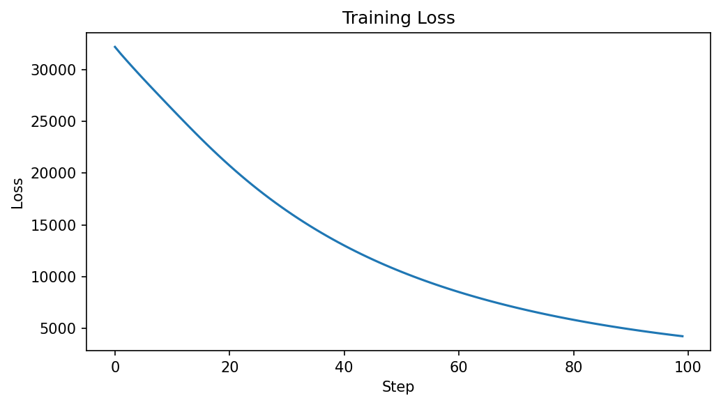
The loss decreases from 32,236 to 4,208 over 100 steps, confirming
the soft k-means objective is being minimized.
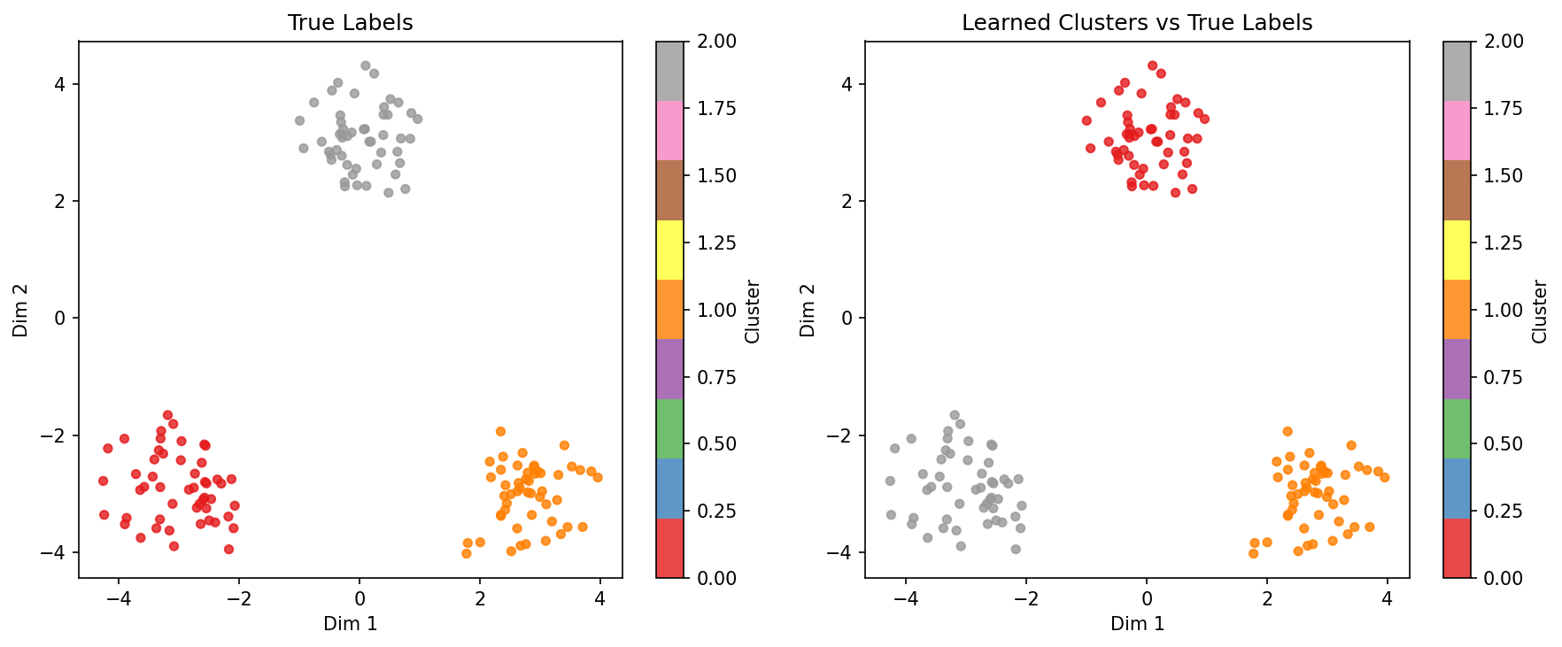
Cluster assignments: (150, 3)
Training loss: 32236.27 -> 4208.34
Accuracy: 100.00%
## Next Steps
- [Related example link]
- [API reference link]
Output Capture Requirements¤
Examples must produce visual and textual outputs that let readers recognize success at a glance. Outputs are captured from actual execution — never hand-written or fabricated.
Visual Outputs (Required)¤
Every example must produce at least one matplotlib figure. Figures are the primary evidence that the example works. Common patterns:
| Example type | Minimum figures |
|---|---|
| Basic (single operator) | 1 figure: output visualization (heatmap, scatter, bar chart) |
| Intermediate (multi-operator) | 2-3 figures: per-step outputs + parameter sweep |
| Advanced (pipeline/ecosystem) | 3-4 figures: pipeline stages + metrics + experiments |
In the .py source, use plt.show() so figures render in notebooks. Also
use plt.savefig() to write each figure to a deterministic path:
import matplotlib.pyplot as plt

# After computing results...
fig, ax = plt.subplots(figsize=(7, 4))
ax.plot(losses)
ax.set_xlabel("Step")
ax.set_ylabel("Loss")
ax.set_title("Training Loss")
plt.tight_layout()
plt.savefig("docs/assets/examples/singlecell/clustering_loss.png", dpi=150, bbox_inches="tight")
plt.show()
Asset Organization¤
Place captured figures under docs/assets/examples/, mirroring the example
directory structure:
docs/assets/examples/
  basic/
    operator_pattern_assignments.png
  singlecell/
    clustering_loss.png
    clustering_scatter.png
    imputation_heatmaps.png
    imputation_correlation.png
    ...
  pipelines/
    pipeline_overview.png
  ecosystem/
    scvi_elbo.png
    scvi_latent.png
Textual Outputs (Required)¤
Every example must print key results in a structured format:
- Tensor shapes for all outputs:
print(f"Output shape: {result['key'].shape}") - Key scalar values: loss, accuracy, correlation, metric scores
- Verification results: gradient non-zero, JIT matches eager
Format textual output as compact, labeled lines — not raw dumps:
# Good: structured, scannable
print(f"Cluster assignments: {assignments.shape}")
print(f"Training loss: {losses[0]:.2f} -> {losses[-1]:.2f}")
print(f"Accuracy: {accuracy:.1%}")

# Bad: unstructured wall of text
print(result)
print(grads)
Linking from Doc Pages¤
In the companion docs/examples/.../*.md page, embed figures with alt text
and include textual output in fenced code blocks:
## Results
The training loss decreases steadily over 100 steps:

After training, clusters separate cleanly in 2D projection:
Expected output:
Cluster assignments: (150, 3)
Training loss: 32236.27 -> 4208.34
Accuracy: 100.00%
Generating Assets¤
The recommended workflow for capturing outputs:
source ./activate.sh

# 1. Run the example (produces .png files via savefig)
uv run python examples/singlecell/clustering.py

# 2. Sync the notebook pair
uv run python scripts/jupytext_converter.py sync examples/singlecell/clustering.py

# 3. Verify assets exist
ls docs/assets/examples/singlecell/clustering_*.png
Avoid long unstructured logs in docs pages.
Visual and Narrative Style¤
Write example docs for comprehension, not marketing.
Use:
- concrete section titles (e.g., "Training Loss" not "Results")
- short explanatory paragraphs between figures (1-3 sentences)
- code excerpts with commentary — show the key 5-10 lines, not the whole file
- embedded figures with descriptive alt text
- fenced textual output blocks for key scalar results
- direct statements about tradeoffs and limitations
Avoid:
- vague hype ("powerful", "state-of-the-art")
- unexplained jargon
- giant code dumps with no framing
- duplicated prose between the docs page and the example source
- figures without interpretation — every figure needs a sentence explaining what the reader should observe
Example Difficulty Tiers¤
Basic (5-10 minutes)¤
Single-operator examples. One config, one apply(), one gradient check.
Target audience: first-time DiffBio users.
Examples: DNA encoding, simple alignment, molecular fingerprints, single-cell clustering, quality filtering.
Intermediate (10-20 minutes)¤
Multi-operator workflows. Two or three operators chained, with training loop or evaluation. Target audience: users building custom pipelines.
Examples: batch correction + clustering, trajectory inference + fate analysis, VAE normalization + cell type annotation.
Advanced (20-40 minutes)¤
Full pipeline composition with ecosystem integration (calibrax metrics, artifex losses, opifex training). Training loops, benchmarking, comparison against reference tools. Target audience: researchers adapting DiffBio for their data.
Examples: scVI benchmark, multi-omics integration pipeline, spatial transcriptomics domain analysis, GRN inference with SCENIC comparison.
Maintenance Rules¤
When an example changes, review all three surfaces:
- example
.py - paired
.ipynb docs/examples/...page
Also update contributor-facing surfaces if the workflow contract changed:
examples/README.mdCONTRIBUTING.mddocs/development/contributing.md
Review Checklist¤
Before merging an example:
Execution
- [ ] the example runs with source ./activate.sh
- [ ] the example runs with uv run python examples/path/to/example.py
- [ ] device requirements are stated accurately
- [ ] the .ipynb pair was synced via scripts/jupytext_converter.py sync
Visual Outputs
- [ ] at least one matplotlib figure is produced
- [ ] figures are saved via plt.savefig() to docs/assets/examples/...
- [ ] saved figures exist on disk after running the example
- [ ] the docs page embeds all figures with  and alt text
- [ ] every embedded figure has a short interpretation sentence
Textual Outputs - [ ] output shapes are printed for all result tensors - [ ] key scalar values are printed (loss, accuracy, metrics) - [ ] gradient verification prints non-zero and finite checks - [ ] JIT verification prints match result - [ ] the docs page includes expected textual output in fenced blocks
Content
- [ ] the docs page matches the current source
- [ ] imports use the supported DiffBio public API surface
- [ ] commands use uv
- [ ] notebook and docs do not teach hidden backend forcing
- [ ] the example teaches a concrete bioinformatics concept
- [ ] differentiability is demonstrated (gradient flow check)
- [ ] JIT compilation is demonstrated
- [ ] ecosystem building blocks are used where appropriate (calibrax, artifex, opifex)
- [ ] synthetic data is generated (no external file dependencies)
Recommended Author Workflow¤
source ./activate.sh

# 1. create or edit the Python source
$EDITOR examples/path/to/example.py

# 2. create the asset directory (if new example)
mkdir -p docs/assets/examples/domain/

# 3. run the example (produces figures via plt.savefig + verifies execution)
uv run python examples/path/to/example.py

# 4. verify figures were generated
ls docs/assets/examples/domain/*.png

# 5. regenerate the notebook pair from the Python source
uv run python scripts/jupytext_converter.py sync examples/path/to/example.py

# 6. write/update the docs page (embed figures and textual outputs)
$EDITOR docs/examples/path/to/example-name.md

# 7. verify docs build (confirms figure paths resolve)
uv run mkdocs build
Related Files¤
docs/examples/templates/example_template.py— DiffBio example templatescripts/jupytext_converter.py— py/ipynb conversion and sync utilityexamples/README.md— index of runnable examplesCONTRIBUTING.mddocs/development/contributing.md