HMM Sequence Model

This example demonstrates how to use DiffBio's differentiable Hidden Markov Model for sequence analysis.

Overview

Hidden Markov Models (HMMs) are powerful tools for:

• Gene finding (coding/non-coding regions)
• Chromatin state annotation
• Profile search (protein domains)
• Sequence labeling

DiffBio implements a fully differentiable HMM using the forward algorithm with logsumexp for numerical stability.

Prerequisites

import jax
import jax.numpy as jnp
from flax import nnx

from diffbio.operators.statistical import DifferentiableHMM, HMMConfig

Step 1: Configure the HMM

# Create a 3-state HMM for gene finding
# States: intergenic (0), exon (1), intron (2)
# Emissions: DNA bases A=0, C=1, G=2, T=3

config = HMMConfig(
    num_states=3,        # Hidden states
    num_emissions=4,     # Observation symbols (DNA bases)
    temperature=1.0,     # Temperature for softmax
)
rngs = nnx.Rngs(42)
hmm = DifferentiableHMM(config, rngs=rngs)

print(f"Number of states: {config.num_states}")
print(f"Number of emissions: {config.num_emissions}")

Output:

Number of states: 3
Number of emissions: 4

Step 2: Create Observation Sequence

# DNA sequence encoded as integers: A=0, C=1, G=2, T=3
observations = jnp.array([0, 1, 2, 3, 0, 1, 2, 3, 0, 0, 1, 1, 2, 2, 3, 3])

print(f"Observation sequence: {observations.tolist()}")
print(f"Sequence length: {len(observations)}")

Output:

Observation sequence: [0, 1, 2, 3, 0, 1, 2, 3, 0, 0, 1, 1, 2, 2, 3, 3]
Sequence length: 16

Step 3: Compute Likelihood and Posteriors

# Apply HMM
data = {"observations": observations}
result, _, _ = hmm.apply(data, {}, None)

log_likelihood = result["log_likelihood"]
posteriors = result["state_posteriors"]

print(f"Log likelihood: {float(log_likelihood):.4f}")
print(f"Posteriors shape: {posteriors.shape}")

Output:

Log likelihood: -22.1816
Posteriors shape: (16, 3)

Step 4: Analyze State Posteriors

# Show state posteriors for first few positions
print("\nState posteriors (first 5 positions):")
state_names = ["Intergenic", "Exon", "Intron"]
for i in range(5):
    probs = posteriors[i]
    print(f"  Position {i}: ", end="")
    for j, name in enumerate(state_names):
        print(f"{name[:3]}={float(probs[j]):.3f} ", end="")
    print()

Output:

State posteriors (first 5 positions):
  Position 0: Int=0.331 Exo=0.371 Intr=0.298
  Position 1: Int=0.345 Exo=0.321 Intr=0.334
  Position 2: Int=0.326 Exo=0.381 Intr=0.294
  Position 3: Int=0.335 Exo=0.349 Intr=0.315
  Position 4: Int=0.331 Exo=0.356 Intr=0.313

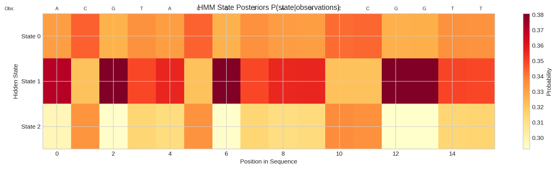
State posteriors P(state|observations) for each position in the sequence. Each column shows the probability distribution over hidden states.

Random Initialization

With random parameters, posteriors are roughly uniform. After training on labeled data, the HMM learns meaningful state assignments.

Understanding the HMM

Model Parameters

The HMM has three parameter matrices:

1. Initial distribution \(\pi\): \(P(\text{state}_0 = i)\)
2. Transition matrix \(A\): \(P(\text{state}_t = j | \text{state}_{t-1} = i)\)
3. Emission matrix \(B\): \(P(\text{obs}_t = k | \text{state}_t = i)\)

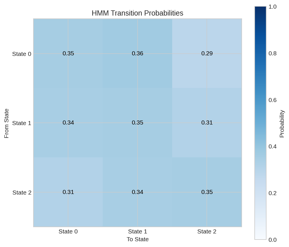
Transition probability matrix showing P(next state | current state). After training, patterns emerge such as high self-transition probability for stable states.

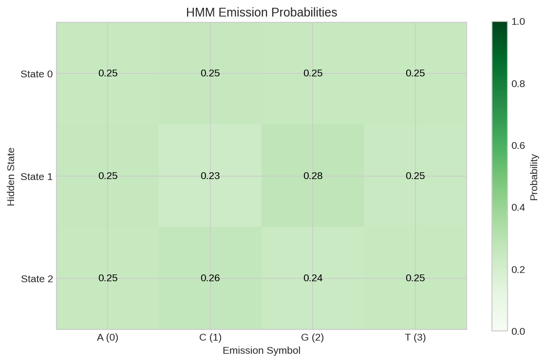
Emission probability matrix showing P(observation | state). Different states learn to emit different DNA base patterns.

Forward Algorithm

The forward algorithm computes \(P(\text{observations} | \text{model})\) efficiently:

\[\alpha_t(j) = P(o_1, ..., o_t, s_t = j)\]

In log space (for numerical stability): $\(\log \alpha_t(j) = \text{logsumexp}_i(\log \alpha_{t-1}(i) + \log A_{ij}) + \log B_{j,o_t}\)$

State Posteriors

The forward-backward algorithm computes:

\[P(s_t = i | o_1, ..., o_T)\]

These posteriors indicate the most likely state at each position.

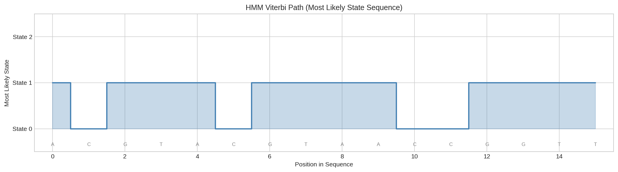
Most likely state sequence (Viterbi path) showing the predicted hidden state at each position based on posterior probabilities.

Differentiability

The HMM is fully differentiable, enabling gradient-based training:

def loss_fn(hmm, data):
    """Negative log-likelihood loss."""
    result, _, _ = hmm.apply(data, {}, None)
    return -result["log_likelihood"]

# Compute gradients
grads = nnx.grad(loss_fn)(hmm, data)
print("Differentiable: Yes (gradient computation successful)")

Output:

Differentiable: Yes (gradient computation successful)

Training the HMM

Train on labeled sequences (e.g., annotated genes):

import optax

# Create optimizer
optimizer = optax.adam(learning_rate=0.01)
opt_state = optimizer.init(nnx.state(hmm))

# Training step
def train_step(hmm, data, opt_state):
    def loss_fn(model):
        result, _, _ = model.apply(data, {}, None)
        return -result["log_likelihood"]

    loss, grads = nnx.value_and_grad(loss_fn)(hmm)
    updates, opt_state = optimizer.update(grads, opt_state)
    nnx.update(hmm, updates)
    return loss, opt_state

# Training loop (pseudocode)
# for epoch in range(epochs):
#     for batch in dataloader:
#         loss, opt_state = train_step(hmm, batch, opt_state)

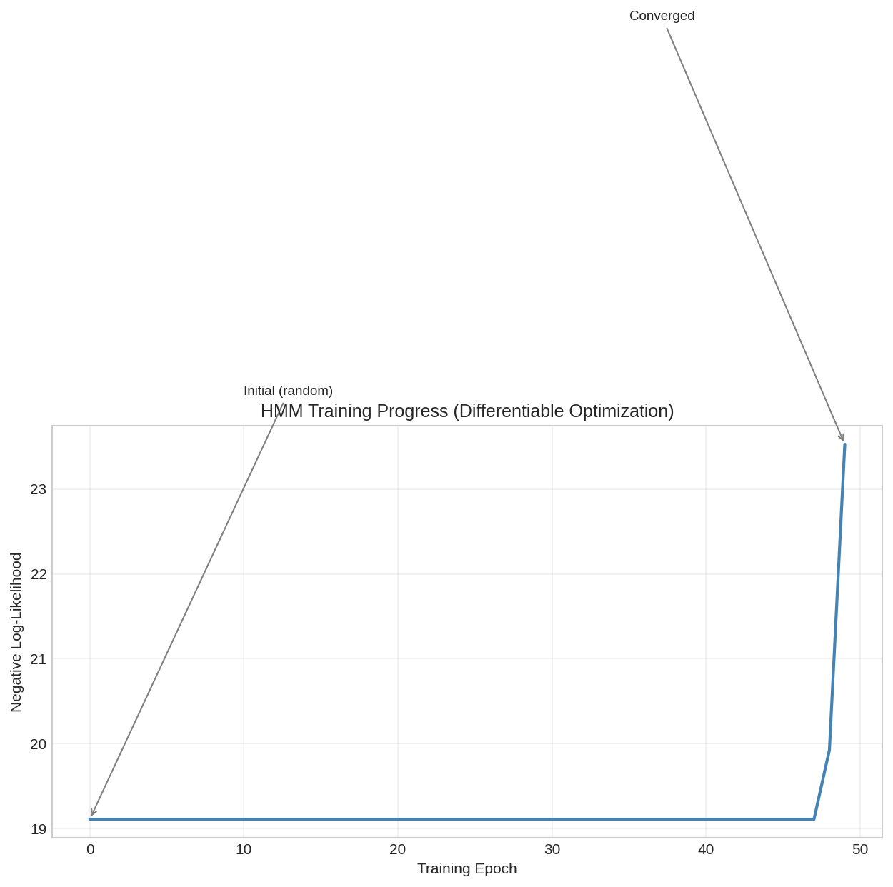
HMM training progress showing negative log-likelihood decreasing over epochs. The differentiable implementation enables gradient-based optimization.

Soft Observations

For uncertain observations (e.g., from sequencing), use soft probabilities:

# Soft observations: probability distribution over bases at each position
soft_obs = jnp.array([
    [0.9, 0.05, 0.03, 0.02],  # Likely A
    [0.1, 0.7, 0.1, 0.1],    # Likely C
    [0.05, 0.05, 0.85, 0.05], # Likely G
    # ...
])

# Use forward_soft for soft observations
log_prob = hmm.forward_soft(soft_obs)

Applications

Application	States	Emissions
Gene finding	Intergenic, Exon, Intron	DNA bases
Chromatin states	Active, Poised, Repressed	Histone marks
CpG islands	CpG-rich, CpG-poor	Dinucleotides
Protein domains	Domain types	Amino acids

Configuration Options

Parameter	Description	Default
num_states	Number of hidden states	3
num_emissions	Number of observation symbols	4
temperature	Softmax temperature	1.0
learnable_transitions	Learn transition matrix	True
learnable_emissions	Learn emission matrix	True

Next Steps

• DNA Encoding - Encode sequences for HMM
• RNA Structure - Structure-based sequence analysis
• Single-Cell Clustering - Clustering for different domains