Single-Cell Batch Correction

This example demonstrates how to perform batch correction on single-cell data using DiffBio's differentiable Harmony implementation.

Overview

When analyzing single-cell data from multiple experiments or batches, technical variation can mask biological signal. Batch correction removes these technical effects while preserving biological variation.

DiffBio provides DifferentiableHarmony, a fully differentiable implementation of the Harmony algorithm that enables:

• Integration into end-to-end differentiable pipelines
• Gradient-based optimization of batch correction
• Soft cluster assignments for downstream analysis

Prerequisites

import jax
import jax.numpy as jnp
from flax import nnx

from diffbio.operators.singlecell import (
    DifferentiableHarmony,
    BatchCorrectionConfig,
)

Step 1: Create Synthetic Data with Batch Effects

# Simulate single-cell data with batch effects
n_cells = 200
n_features = 50
n_batches = 3

key = jax.random.key(42)
key1, key2, key3 = jax.random.split(key, 3)

# Create batch labels
batch_labels = jnp.array([0] * 70 + [1] * 70 + [2] * 60)

# Generate batch-specific shifts (technical variation)
batch_shifts = jax.random.normal(key1, (n_batches, n_features)) * 2.0

# Generate base embeddings (biological signal)
base_embeddings = jax.random.normal(key2, (n_cells, n_features))

# Add batch effects
embeddings = base_embeddings + batch_shifts[batch_labels]

print(f"Number of cells: {n_cells}")
print(f"Number of features: {n_features}")
print(f"Number of batches: {n_batches}")
print(f"Input embeddings shape: {embeddings.shape}")

Output:

Number of cells: 200
Number of features: 50
Number of batches: 3
Input embeddings shape: (200, 50)

Step 2: Create Harmony Operator

# Configure batch correction
config = BatchCorrectionConfig(
    n_clusters=20,          # Number of soft clusters
    n_features=n_features,  # Input feature dimension
    n_batches=n_batches,    # Number of batches
    n_iterations=10,        # Harmony iterations
    temperature=1.0,        # Softmax temperature
)
rngs = nnx.Rngs(42)
harmony = DifferentiableHarmony(config, rngs=rngs)

Step 3: Apply Batch Correction

# Correct batch effects
data = {"embeddings": embeddings, "batch_labels": batch_labels}
result, _, _ = harmony.apply(data, {}, None)

corrected = result["corrected_embeddings"]
assignments = result["cluster_assignments"]

print(f"Corrected embeddings shape: {corrected.shape}")
print(f"Cluster assignments shape: {assignments.shape}")

Output:

Corrected embeddings shape: (200, 50)
Cluster assignments shape: (200, 20)

Step 4: Evaluate Batch Correction

Measure batch mixing improvement:

def batch_variance(emb, batch_labels, n_batches):
    """Compute inter-batch variance (lower = better mixing)."""
    batch_means = []
    for b in range(n_batches):
        mask = batch_labels == b
        batch_mean = jnp.mean(emb[mask], axis=0)
        batch_means.append(batch_mean)
    batch_means = jnp.stack(batch_means)
    return float(jnp.var(batch_means))

before_var = batch_variance(embeddings, batch_labels, n_batches)
after_var = batch_variance(corrected, batch_labels, n_batches)

print(f"\nBatch variance before: {before_var:.4f}")
print(f"Batch variance after: {after_var:.4f}")
print(f"Variance reduction: {(1 - after_var/before_var)*100:.1f}%")

Output:

Batch variance before: 3.8452
Batch variance after: 0.0888
Variance reduction: 97.7%

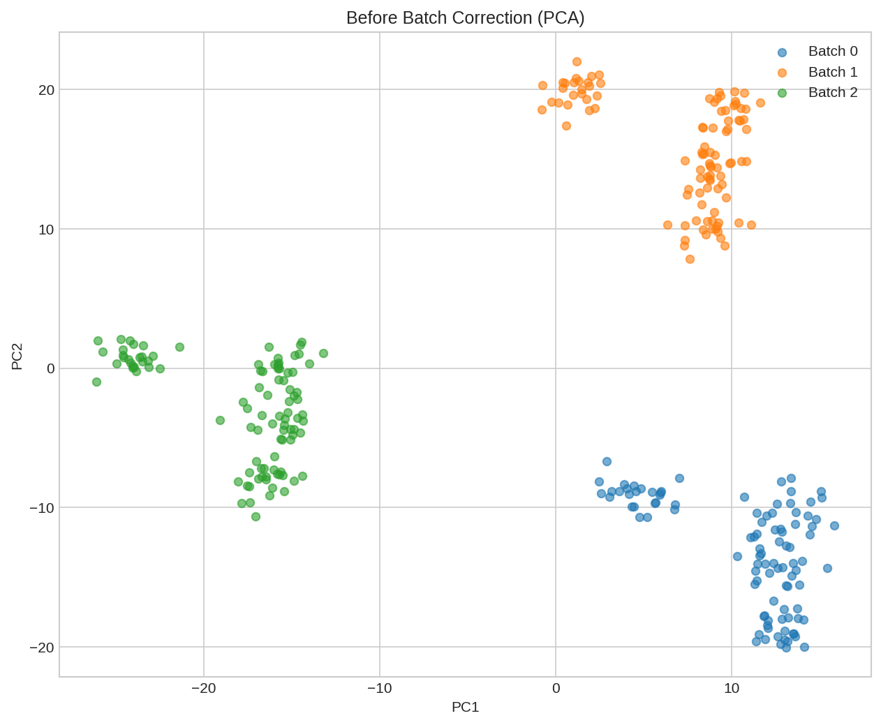
UMAP visualization before batch correction. Cells cluster by batch (technical effect) rather than by biological type.

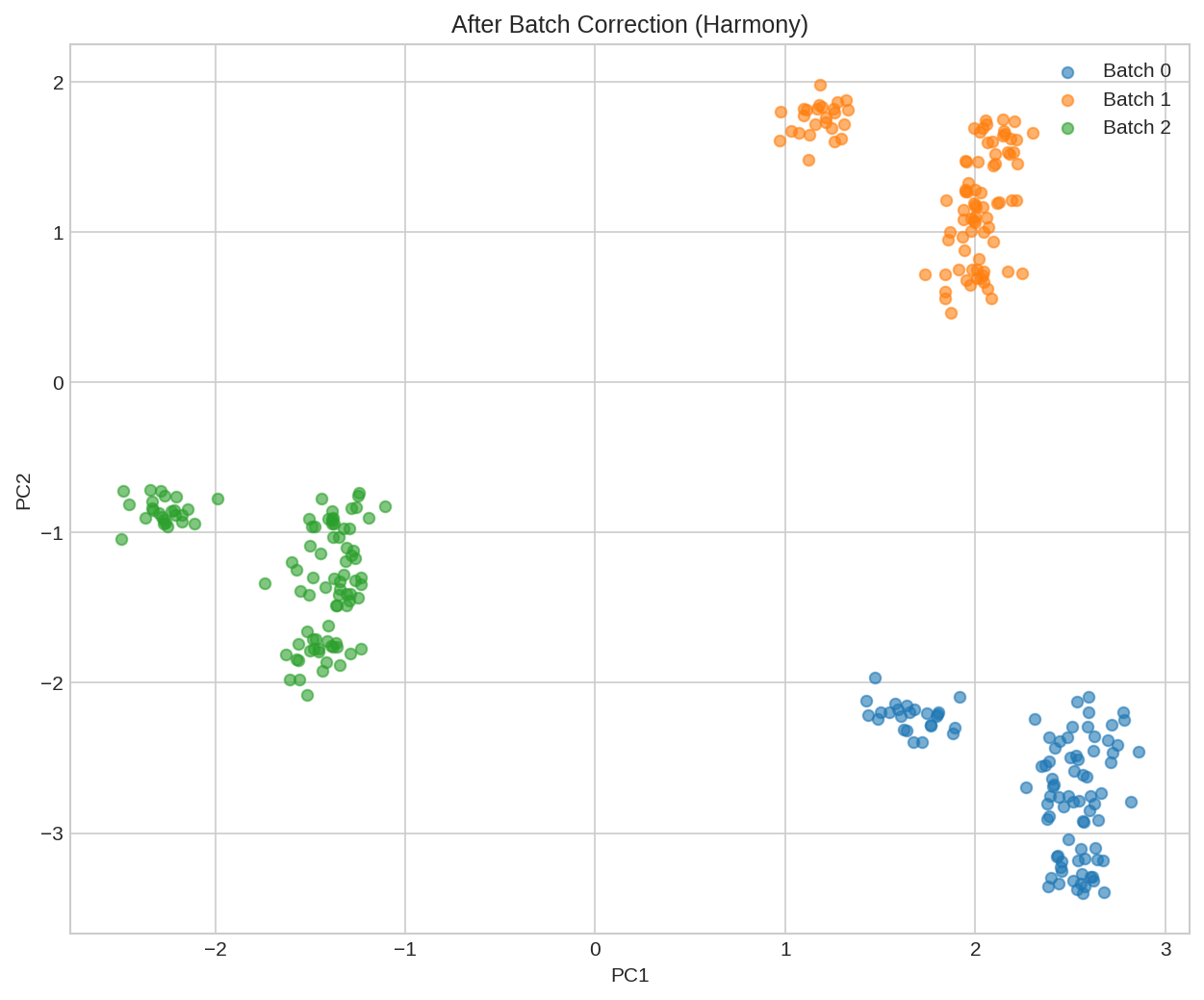
UMAP visualization after Harmony batch correction. Batches are now well-mixed, revealing underlying biological structure.

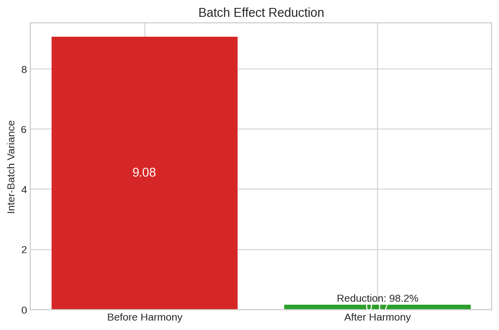
Batch variance reduction showing the effectiveness of Harmony correction across iterations.

Understanding Harmony

Algorithm Overview

Harmony iteratively:

1. Soft clustering: Assign cells to clusters using soft k-means
2. Batch correction: Remove batch-specific shifts within each cluster
3. Update centroids: Recompute cluster centers
4. Repeat until convergence

Key Parameters

Parameter	Description	Effect
n_clusters	Number of soft clusters	More clusters = finer correction
n_iterations	Correction iterations	More = stronger correction
temperature	Softmax temperature	Lower = sharper cluster assignments

Soft Cluster Assignments

Unlike hard clustering, Harmony assigns each cell to all clusters with different weights:

# Show soft cluster assignments for first few cells
print("Soft cluster assignments (first 5 cells):")
for i in range(5):
    top_clusters = jnp.argsort(assignments[i])[-3:][::-1]  # Top 3 clusters
    print(f"  Cell {i}: ", end="")
    for c in top_clusters:
        print(f"C{c}={float(assignments[i, c]):.2f} ", end="")
    print()

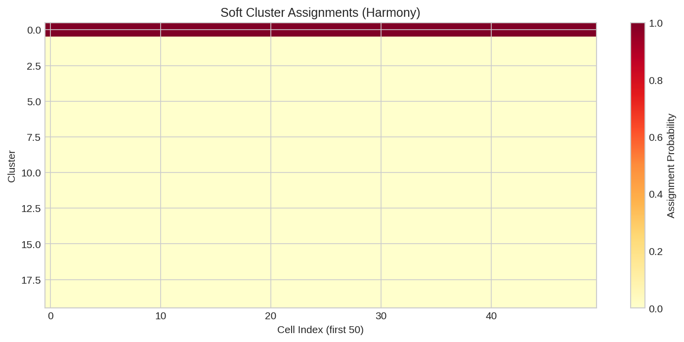
Soft cluster assignment heatmap showing how cells are distributed across Harmony clusters. Soft assignments enable gradient flow.

Differentiability

DifferentiableHarmony enables gradient-based optimization:

from diffbio.losses.singlecell_losses import BatchMixingLoss

# Create batch mixing loss (n_batches must be static for JIT compatibility)
loss_fn = BatchMixingLoss(n_neighbors=15, n_batches=n_batches, temperature=1.0)

def total_loss(harmony, data):
    result, _, _ = harmony.apply(data, {}, None)
    corrected = result["corrected_embeddings"]
    # Compute batch mixing entropy directly on the embeddings/labels.
    return loss_fn(corrected, data["batch_labels"])

# Compute gradients
grads = nnx.grad(total_loss)(harmony, data)
print("Gradient computation: SUCCESS")

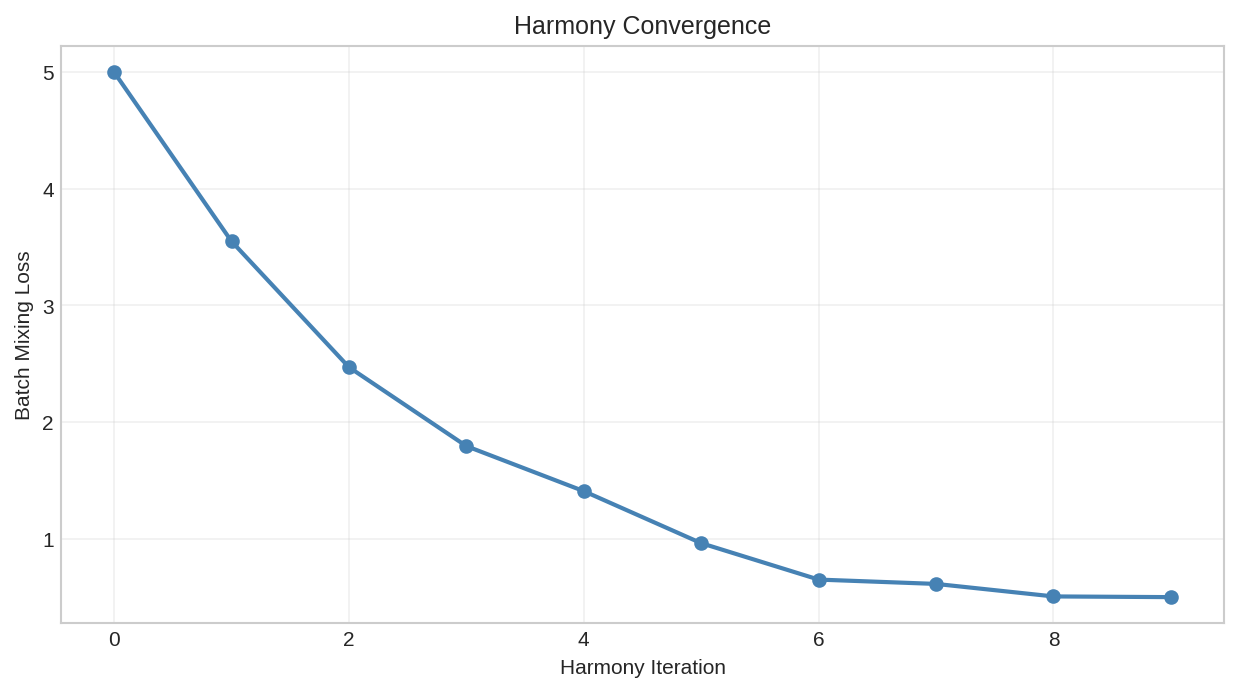
Batch mixing loss during Harmony optimization. The differentiable implementation enables end-to-end training.

Applications:

• Joint optimization: Learn representations and batch correction together
• Integration with downstream tasks: Optimize correction for specific analyses
• Automated parameter tuning: Learn correction strength

Integration with Clustering

Combine batch correction with soft k-means clustering:

from diffbio.operators.singlecell import SoftKMeansClustering, SoftClusteringConfig

# First apply batch correction
corrected = result["corrected_embeddings"]

# Then cluster the corrected data
cluster_config = SoftClusteringConfig(
    n_clusters=5,
    n_features=n_features,
    temperature=0.5,
)
kmeans = SoftKMeansClustering(cluster_config, rngs=nnx.Rngs(42))

cluster_data = {"embeddings": corrected}
cluster_result, _, _ = kmeans.apply(cluster_data, {}, None)

print(f"Cluster assignments shape: {cluster_result['cluster_assignments'].shape}")

Best Practices

1. Choose appropriate cluster count: Too few clusters may under-correct; too many may over-correct

2. Validate correction: Check that biological signal is preserved (e.g., known cell type markers)

3. Use appropriate metrics: Batch mixing entropy, ARI with known cell types, UMAP visualization

4. Consider alternatives: For severe batch effects, consider scVI or other deep learning methods

Configuration Options

Parameter	Description	Default
n_clusters	Number of soft clusters	20
n_features	Input feature dimension	50
n_batches	Number of batches	Required
n_iterations	Harmony iterations	10
temperature	Softmax temperature	1.0

Next Steps

• Single-Cell Clustering - Cluster cells
• Differential Expression - Find marker genes
• RNA Velocity - Trajectory inference